It’s official: the LabNBook plugin for Moodle is now in the Plugin Directory de Moodle. The latest version (1.1.4) was released today.
What does this mean? The plugin has been validated by Moodle. Administrators of Moodle platforms at universities are therefore more inclined to install the plugin on the platform they administer.
What does this plugin do? It creates a link between your university’s Moodle and a LabNBook platform. More information here and here.
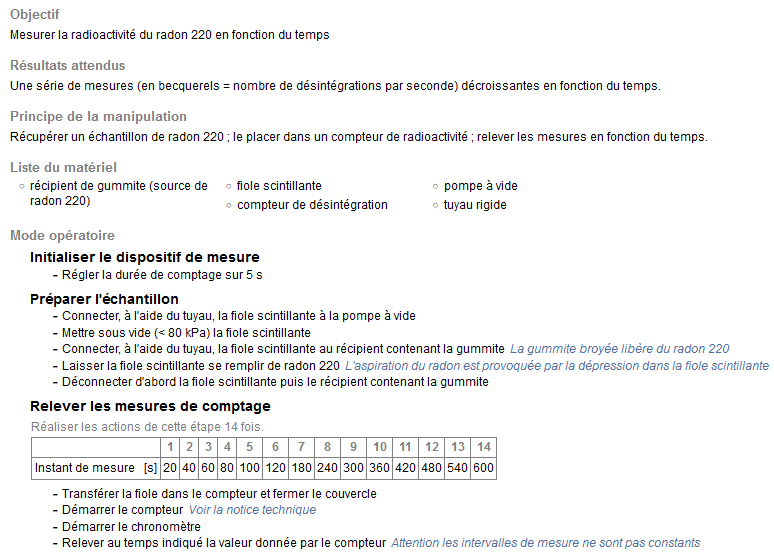
The tool’s interface has changed a little, and the protocol looks more like a “classic” laboratory protocol. We hope that the tool is more mature and easier for students to use.
The most important new feature is for teachers. The new tool makes it possible to propose experimental design activities to students. From a pedagogical point of view, we are convinced that such an activity is beneficial to the understanding of the experiment carried out in the lab. The new tool makes it possible to create pre-structured protocols to support the design of the experiment for students.
A word of advice: to configure the protocol labdoc, you need to be familiar with the basic protocol tool (the one accessible to students by default).
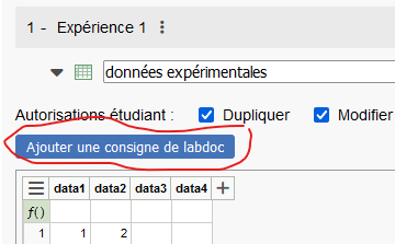
The first new feature lets you add labdoc-level instructionsto a mission.
Currently, instructions are limited to the report parts. If teachers want to provide more specific instructions for a labdoc, they can write directly in the labdoc, but this leads to confusion: the instructions area is not separated from the students’ writing area. And these instructions can be deleted by the students and thus lost in the course of the work…
So we’ve added the possibility for mission designers to add “labdoc instructions” when they edit a mission:
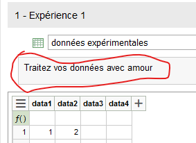
In their report, students can view this instruction by displaying the assignments in the report section or by editing the labdoc :
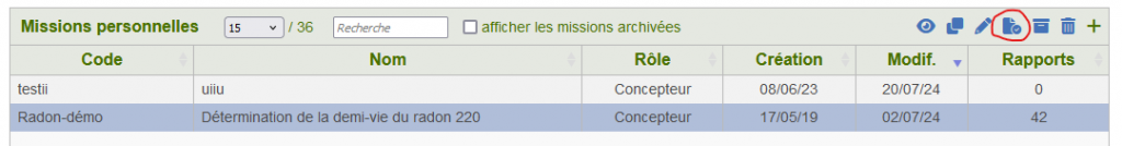
The second new feature is the “teacher report” for each mission. This teacher report can be a solution report to share within a team of teachers, or a report containing “correction” labdocs that you can import into your students’ reports when they have completed their work. Unlike the “Test” report, the “Teachers” report is saved permanently. Only mission designers can modify it. Tutors can only view it. With this new feature, teachers will hardly ever need to use their “student space” again.
Where can is this report? In the “Missions” tab, click on a mission and a new icon will appear in the top right-hand corner of the table:
These are the new LabNBook features that many teachers have been asking for.
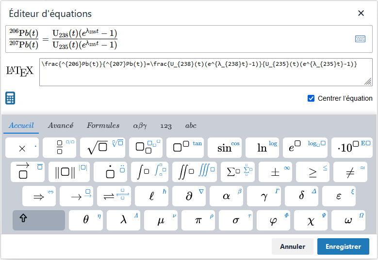
If there’s one aspect of LabNBook that students dislike more than paper documents, it’s writing equations!
And with good reason: writing an equation is always faster on paper… even if you are the king of Latex.
3 years ago, we integrated a tool for writing equations, with a choice of a Latex editor or a graphical interface. This was a first step in the right direction, but unfortunately the tool remained rather buggy and didn’t always produce very comprehensible Latex.
Some time ago, a new, more robust open-source solution emerged: MathLive. We have adapted it to meet the needs of our students. It’s now available on the LabNBook server.
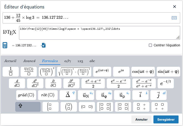
As well as making the tool more sophisticated, we’ve included two time-saving features for students:
A “formulas” menu lets you write some of the classic formulas found in our training courses with a single click.
A button displays the result of the calculation, so you don’t have to use the calculator. Please note, however, that the Latex must be well-formed for the calculation to take place…
Please don’t hesitate to give us any feedback you may have, especially if you notice any missing symbols or formulas, or if you find any of our choices questionable. We’ll do our best to ensure that writing equations on a digital tool takes as little time as possible.
This summer, we implemented the new version of the data processing tool after a complete rewrite of its code.
Let’s start with user-friendliness, as the differences between our tool and the usual spreadsheets may have confused some people. Let’s face it: our tool is not a spreadsheet, as it forces data to be organized in columns. Without drastically changing its interface, we have made some fifteen ergonomic improvements. In a word: the tool is more accomplished.
Let’s move on to the new features:
Cutting and pasting from the previous version was, at best, difficult to use! We’ve completely reworked it. It is now possible to select cells by dragging, or by using the Shift/Maj key at the same time as clicking with the mouse. Then use the classic CTRL-C/X/V or the top-left menu. The only fly in the ointment is that Firefox is (too) secure; to use cut-and-paste in this browser, you need to authorize it via a setting that we explain in a message in case of blockage.
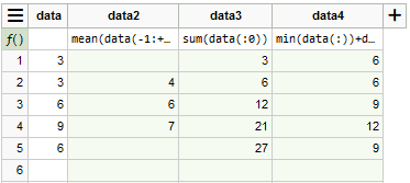
We’ve allowed Math.js functions using a list of values to be used in column formulas. To select values within a data column, use the syntax data(n:m), where n and m are RELATIVE indices relative to the current line. If n is omitted, the list starts at the first row of the column; if m is omitted, the list ends at the last non-empty row of the column. Examples to explain:
mean(data(-1:+1)) calculates a moving average on the data column with 3 values;
sum(data(:0)) calculates the cumulative sum on the data column;
min(data(:)) returns the minimum value of the data column.
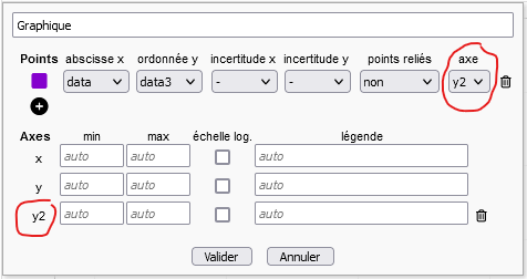
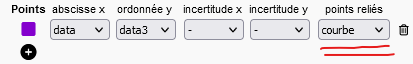
You can now add 2 y-axes to a graph. In the graph parameters, click on the (+) below the axes: a y2 axis appears. For each series of points plotted, you can choose whether to use the y or y2 axis.
It is now possible to connect experimental points by segments or a smoothed curve in the graphs. We were very reluctant to add this feature, which some people had requested. In the end, it has been added, although there is a risk of confusion between a smoothed curve and a model defined by a parametric function: this will be an opportunity to discuss the difference between the two with your students!
We have modified the distance indicators between a parametric function and experimental points. If ALL experimental points have an uncertainty (in y or x, the uncertainty in x being transferred to y according to the slope of the function), X² is used; otherwise, sigma is used. To find out which formula has been applied and the number of points used to calculate the indicator, position your mouse over a calculated value: a speech bubble will provide you with this information. Please note: once a parametric function has been defined, if several sets of points are displayed, you must now select the points it models. Only the distance between these points and the model is calculated.
The most important new feature is the automatic adjustment of parameterized functions to experimental points. By default, this function is not activated for students. In fact, manual adjustment is a pedagogical feature of our tool: by manually adjusting parameters, students can see their effect on the model and understand their scope. But for some students who have understood all this, adjustment can seem time-consuming. Here’s how it works :
The teacher authorizes automatic adjustment at the mission level (“Missions” tab, edit mission, option accessible at the beginning of “Report structure and contents”: “Authorize automatic adjustment for all dataset labdocs”).
For each parameterized function, the student is then presented with a new button for automatic adjustment.
If a parameter is not to be adjusted, click on its name to fix it (same for releasing it).
It may sometimes be necessary to give an initial value to the parameters for the fitting algorithm to converge.
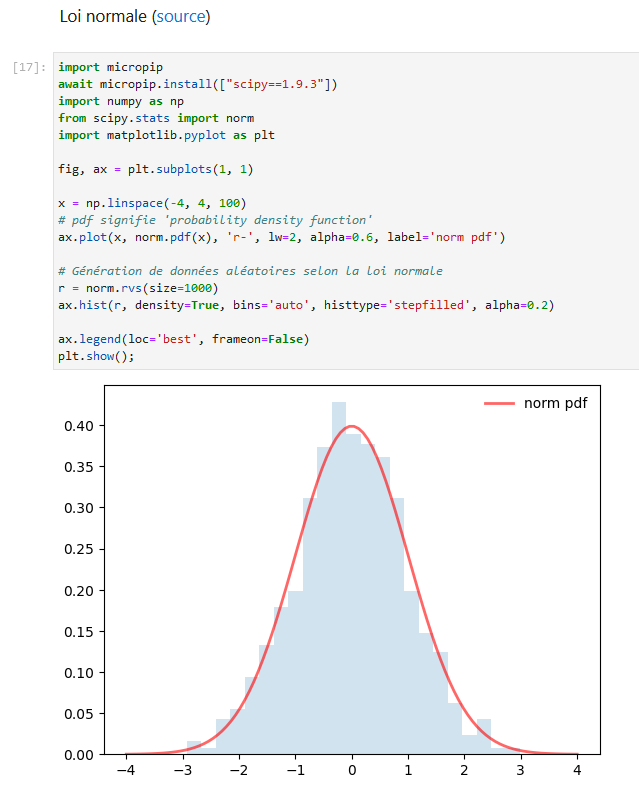
LabNbook is now officially equipped with code labdocs. These new labdocs enable you to write and execute Python code. Your students will be able to go even further in manipulating and representing data during their scientific projects.
No installation is necessary, as labdocs code runs directly in the browser thanks to JupyterLite: tested under Chrome and Firefox by our valiant beta-testers, many thanks to them!
To help you get to grips with JupyterLite, Sébastien (who carried out the development) has produced a public mission called LDcode (to consult it: Mission tab > click on the LDcode mission > click on the eye). This mission can be seen as a user manual in the form of a gallery of examples using the most common Python libraries. Pick and choose what interests you, because it’s 64 pages in PDF format! If you wish to reuse a labdoc from this mission, simply duplicate the mission to make it your own, and the labdoc will be available for import into your missions.